Method of Estimating the Basic Failure Rate and Deriving the Failure Mode and Failure Mode Distribution Rate for Evaluating Random Hardware Failure

Copyright Ⓒ 2020 KSAE / 177-05
This is an Open-Access article distributed under the terms of the Creative Commons Attribution Non-Commercial License(http://creativecommons.org/licenses/by-nc/3.0) which permits unrestricted non-commercial use, distribution, and reproduction in any medium provided the original work is properly cited.
Abstract
Products containing hardware parts with ASIL B or higher levels must perform quantitative assessments of random hardware failures to ensure that they are within the target values. The FMEDA technique is used for this quantitative assessment. To perform FMEDA, input parameters like basic failure rate values, failure mode and failure mode distribution rates for safety-related components, and diagnostic coverage values for safety mechanisms must be prepared. This paper deals with the method of calculating the basic failure rate, deriving the failure mode, and calculating of the failure mode distribution, excluding the diagnostic coverage value of the safety mechanism.
Keywords:
Functional safety, ISO 26262, Random hardware failure, Base failure rate, Failure mode, Failure mode distribution rate, Failure mode effects and diagnostics analysis, Quantitative safety analysis1. Introduction
To perform quantitative evaluation of random hardware failures, as required for functional safety under ISO 26262, the following must be performed:1)
1) evaluation of the hardware architectural metrics; and
2) residual risk assessment for safety goal violation.
The first, “evaluation of the hardware architectural metrics,” is designed to check whether the single-point fault rate and the multi-point latent fault rate present in the hardware to be analyzed are within the allowable range of values, and the evaluation unit is %.
The second, “residual risk assessment for safety goal violation,” is for checking whether the residual risk of safety goal violation is sufficiently low for the hardware to be analyzed, and the evaluation unit is Fit. For this evaluation, ISO26262-5:2018 provides two alternative methods: probabilistic metrics for random hardware failure(PMHF) and evaluation of each cause of safety goal violation(EEC). “Residual risk assessment for safety goal violation” uses either PMHF or EEC.1) The evaluation is usually performed using PMHF, a global probability approach, unless otherwise requested by the customer.
Under the current situation, failure mode effects and diagnostics analysis(FMEDA) is the only practical means to evaluate both 1) and 2) above among the quantitative safety analysis techniques presented in ISO 26262-10:2018. To perform FMEDA, it is necessary to determine the base failure rate(BFR) value, failure mode, and failure mode distribution rate for the safety-related components present in the circuit under analysis. In addition to this, it is necessary to define a safety mechanism that is a technical solution designed to eliminate or suppress the probable single-point faults and multiple-point latent faults that may violate the safety goals. In particular, the diagnostic coverage value for each fault or failure mode that the defined safety mechanism protects should be calculated.2)
This paper deals with the calculation or derivation of the BFR value, failure mode, and failure mode distribution rate for the hardware components to be analyzed, which are the main input parameters required when performing FMEDA.
2. Base Failure Rate (BFR)
2.1 Definition of BFR
In functional safety ISO26262-1:2018, BFR is defined as “failure rate of a hardware element in a given application use case used as an input to safety analyses.” 1) The unit of failure rate λ (lambda) is Fit, and 1 Fit is 10-9/h. This statistically means the probability of a failure occurring once per billion hours, and it is related to the mean time to failure (MTTF), which is the average failure time, when repair is impossible. That is, as MTTF=1/λ, the life of a product with 1 Fit is 109 h. In the case of semiconductors, these basic BFRs can be classified into a permanent failure rate in which faults are maintained until they are removed or repaired, and a temporary failure rate in which faults are formed and disappear.
For reference, the same unit called “Fit” is used for both the BFR and the PMHF value, which is one of the results of performing FMEDA. These two values, however, are totally distinguished from each other for the following reasons.
BFR, which is used as an input for quantitative safety analysis, is a device-specific failure rate determined not only by the inherent properties of the material but also by various factors associated with the manufacturing process characteristics, the environmental characteristics(e.g., internal and external temperatures), and the operating conditions(e.g., operating cycles).
On the other hand, the PMHF value is a failure rate that reflects the diagnostic coverage value of a safety mechanism that classifies the faults for each failure mode by safety goal, using BFR as an input, and that protects the classified faults. As such, it is a value that varies greatly depending on the set safety goals and safety requirements, safety mechanisms, and design methods.
2.2 Sources for BFR Calculation
According to ISO26262-11:2018, 4.6.1.6, BFR values can be calculated based on the sources cited below.4)
1) Failure rates derived from the following experimental testing:
① high-temperature operating life tests for intrinsic product operation reliability
② temperature, bias, and operating life tests, known as extended life tests
③ convergence characteristic of acceleration tests for screening (to find faults/failures, etc.)
2) Failure rates derived from field accident observations, such as analysis of materials returned from field failures
3) Failure rates estimated from the application of the industry reliability data book or derived and combined with experts’ assessment
In the case of 1), which is based on the reliability evaluation, it is a statistical approach based on the number of failures compared to the sampling, and the failure rate value can be changed according to the test methods. In the case of 2), which is based on the field data, it is a statistical approach based on the number of failures returned from the field compared to the quantity of components being operated in the field, and the failure rate value may be changed according to the operating environment. ISO26262-11:2018 proposes the exponential model method for methods 1) and 2). The model uses the χ²(chi square) statistical function and recommends an around 70 % confidence level.4)
In the case of 3), the permanent failure rate for the hardware parts is calculated using the data displayed in various tables, along with the mathematical modeling for each hardware part according to the industry reliability data book. At this time, various parameters to be entered in the mathematical modeling are selected or obtained according to experts’ judgment.
2.3 Industry Reliability Data Book
The relevant industries provide various industry data books. The typical data books, as presented by ISO26262-5:2018, include SN 29500, IEC 61709, MIL HDBK 217 F notice 2, RIAC HDBK 217 Plus, UTE C80-811, NPRD-2016, EN 50129:2003, Annex C, RIAC FMD-2016, MIL HDBK 338, and FIDES 2009 EdA.1) Of these, the data books that are currently recognized and actively being used by the domestic industries are IEC TR 62380 and SN 29500.
1) RDF-2000 Module(IEC TR 62380): This is a reliability data handbook published by UTE(Union Technique de l' Electricite) and designed to predict the failure rate of electronic devices based on UTE C 80-810. The IEC TR 62380 reliability prediction method, taking into account the effects of a phased mission profile for operating and non-operating components, explains the effects of thermal cycling for component failure rates due to the changes in the ambient temperatures and to the on/off states of the component switches.5) For its advantages, it is optimized to calculate the failure rate of semiconductors. For reference, IEC TR 62380 was withdrawn by IEC in 2017, but with the sector of semiconductors applied in ISO 26262-11:2018, it can be used to predict the semiconductor failure rates.
2) Siemens SN 29500: Developed by Siemens and its affiliates in Germany to be used a unified standard for reliability prediction, SN 29500 is based on IEC 617095) and simplifies the input parameters for calculating failure rates by selecting table data according to the hardware element.
3) IEC 61709: By integrating IEC 61709 2nd edition and IEC TR 62380:2004, the third edition was published in 2017. It provides a guideline for using the failure rate date for the prediction of the reliability of electric and electronic parts, but it does not provide the BFR for hardware parts. It provides a model for converting a failure rate obtained through a means different from one operating condition to another.5)
4) MIL-HDBK-217: This U.S. Department of Defense standard was designed to predict the reliability of electronic parts, and it has been the mainstay for reliability predictions for about 40 years. MIL-HDBK-217 provides two reliability prediction methods, as shown below. 5)
① The method calculating the number of parts: This is the simpler method to use in the early design phase, and it needs information like the quality, quantity, and environment.
② The parts stress method: More complicated, this method needs detailed information on the temperature conditions and electrical stress. It is used in designing hardware and circuits.
5) NPRD 2016: It deals with the failure rates of various items, including machines, electronic and mechanical parts, and assemblies. It provides detailed failure rate data for over 25,000 parts with regard to a vast number of categorized parts grouped by environmental and quality levels.5)
6) FIDES 2009: This is a reliable data book that was developed by a French industrial consortium under the supervision of the French Ministry of Defense. The FIDES methodology, which is based on the physics of failure, provides support through test data, return from the field, and analysis of existing modeling.5)
2.4 Examples of BFR Calculation
This section provides examples of calculating BFR for semiconductor elements according to the electronic parts reliability prediction models IEC TR 62380 and SN29500, as well as examples of calculating BFR for hardware elements using the χ² (chi square) statistical function.
The following are easy-to-understand examples of calculating the BFR of microprocessors provided by IEC TR 62380.6) These examples do not mention several methods of combining the integrated-circuit product group type value λ1 and the semiconductor mastering technology-related vale λ2 according to the various technologies(CPU, memory, peripherals, etc.) implemented in semiconductors, as described in ISO26262-11:2018, 4.6.2.1.1.1.4)
1) Mission profile: Considering the temperatures and operating environment6)
① Overall working time: 500 h
② 3 temperature phases (3 temperature states of vehicles):
- Motor still cold
- Motor warm
- Motor runs with high speed (hot)
③ 3 cycles of operation (3 operating states of vehicles):
- 2 night trips per day
- 4 day trips per day
- 30-day shutdown
2) Mathematical models for semiconductor integrated circuits6):
| (1) |
| (2) |
where
λ1 : per-transistor base failure rate of the integrated circuit family
λ2 : failure rate related to the technology mastering of the integrated circuit
N : number of transistors of the integrated circuit
a : [(year of manufacture) - 1998]
(πt)i : ith temperature factor related to the ith junction temperature of the integrated circuit mission profile
τi : ith working time ratio of the integrated circuit for the ith junction temperature of the mission profile
τon : total working time ratio of the integrated circuit
τoff : time ratio for the integrated circuit in storage (or dormant)
| (3) |
where
πa : influence factor related to the thermal expansion coefficient difference between the mounting substrate and the package material
(πn)i : ith influence factor related to the annual cycles’ number of thermal variations seen by the package, with amplitude ΔTi
ΔTi : ith thermal amplitude variation of the mission profile
λ3 : base failure rate of the integrated circuit package
| (4) |
where
πI : influence factor related to the use of the integrated circuit (interface or not)
λEOS : failure rate related to the electrical overstress in the considered application
3) Information of the analysis target: Microprocessor6)
- Application type: Passenger compartment
- Year of manufacture: 1999
- Technology: Numerical CMOS
- Transistor number: 1.5×10⁶
- Dissipated power by the component: 0.5 W
- Airflow factor: Natural convection
- PQFP 80-pin package
- Mounting substrate: FR4
- This circuit is not an interface.
4) Calculate the λdie value using equation (2).
① To find the λ1 and λ2 values for microprocessors and numerical CMOS, refer to IEC TR 62380 Table 16.6)
⇨ λ1 = 3.4×10⁻⁶, λ 2 = 1.7
② Number of transistors, N = 1.5×10⁶
③ Find the a value according to the year of manufacture.
⇨ a = 1999 - 1998 = 1
④ To find the πt value, first, find the ΔTj (increased junction temperatures) value. For this, one must know the ambient heat resistance of the PQFP 80-pin package. Thus, refer to IEC TR 62380 Table 126) to obtain the following formula:
| (5) |
where
K : airflow factor
S : number of pins
Under the given conditions, K is natural convection, and it is 1.4 according to IEC TR 62380 Table 13.6) Under the given conditions, likewise, S is 80. Therefore, the RTHja value is 67 °C/W.
| (6) |
⑤ Refer to the three state values of temperature provided in the Table 1 mission profile to find the (πt)i value. The temperature factor πt for numerical CMOS is as shown below.6)

IEC TR 62380: Table 11 - Mission profiles for automotives6)
| (7) |
where
A : A = 3480; (Ea=0.3 eV)
tj : junction temperature in °C
| (8) |
where
(tac)i : average ambient temperature of the printed circuit board (PCB) near the components, where the temperature gradient is cancelled
Based on equation (8),
t1 = 27 °C + 34 °C = 61 °C
t2 = 30 °C + 34 °C = 64 °C
t3 = 85 °C + 34 °C = 119 °C
When these are substituted into equation (7) for calculation, the values below are obtained.
(πt)1 = 1.21
(πt)2 = 1.33
(πt)3 = 5.5
⑥ The τi value is provided in the Table 1 mission profile, and the values below are obtained.
τ1 = 0.006
τ2 = 0.046
τ3 = 0.006
⑦ τon the τoff value is likewise provided in the Table 1 mission profile, and the values below are obtained.
τon = 0.058
τoff = 0.942
As disclosed in ISO 26262-11:2018, 4.6.2.1.1.24), however, to calculate the conservative temperature de-rating factor, set τoff to 0.
⑧ Substitute all the above parameters into equation (2) to calculate the λdie value. Then the failure rate of λdie will become 9.25 Fit.
5) Using equation (3), calculate the λpackage value.
① Using equation (9) below, find the πa value.6)
| (9) |
as (substrate) and ac (component) become 16 and 21.5, respectively, according to IEC TR 62380 Table 14. Therefore, the πa value is 1.05.
② Refer to IEC TR 62380 Table 17a to find the λ3 value. Under the given conditions, the λ3 value for PQFP 80 pins is 10.2 Fit. For reference, if the package type and size are not listed in IEC TR 62380 Table 17a, refer to IEC TR 62380 Table 17b to calculate the λ3 value.6)
③ Based on equation (10), find the ΔTi value.6)
| (10) |
where
(tac)average : average temperature during the working phases
(tae)i : average outside ambient temperature surrounding the equipment, during the ith phase of the mission profile
Obtain the average temperature (tac)average value during the operation phase using equation (11).
When calculated by referring to the Table 1 mission profile, the (tac)average value is 35 °C.
| (11) |
To obtain the (tae)i value, refer to IEC TR 62380 Table 8.6) This table indicates that the temperature for the night is 5 °C and the temperature for the day is 15°C in the world climate type. Therefore,
(tae)1 = 5 °C; and
(tae)2 = 15 °C.
Substitute the above values into equation (10) to calculate and obtain the values below.
ΔT1 = {(34 °C/3) + 35 °C} - 5 °C = 41 °C
ΔT2 = {(34 °C/3) + 35 °C} - 15 °C = 31 °C
In addition, ΔT3 is calculated as shown below, by applying the value recorded in the Table 1 mission profile under the given condition of not running vehicles for 30 days in a year.
ΔT3 = 10 °C
④ Obtain the ( πn)i value. The three vehicle operation cycles in a year specified in the Table 1 mission profile are all within 8760 h, so the equation applied to ( πn)i is equation (12) below.6)
| (12) |
⑤ Substitute all the above parameters into equation (3) to calculate the λpackage value. Then the failure rate of λpackage is 126 Fit.
6) Calculate the λ overstress value using equation (4).
① Find the πI value. In the case of microprocessors, they are generally not directly connected to the external environment, so πI = 0.
② Find the λEOS value. IEC TR 623806) does not present λEOS for the electrical environment of vehicles. Instead, you can choose “electronic engineering for private aviation,” so λEOS is 20 Fit.
③ Substitute all the above parameters into equation (4) to calculate the λoverstress value. Then the failure rate of λoverstress is πI × λEOS = 0 Fit.
For reference, the semiconductor devices directly connected to the external environment include a communication transceiver IC, a regulator IC, and the like. As these devices have πI = 1, the λoverstress value is 20 Fit.
1) Finally, the BFR value for microprocessors is calculated as shown below, using equation (1).
λ = 9.25 Fit + 126 Fit + 0 Fit = 135.25 Fit
SN295007) has the advantage of simplifying the input parameters for calculating the failure rate because it uses the table search method. If appropriate data are not available in the table, however, it has to take the trouble of estimating the data value using interpolation or extrapolation. Further, as mentioned in ISO26262-11:2018, 4.6.2.1.2.44), unlike IEC TR 623806), SN295007) does not provide the method of dividing the failure rates into the package failure rate and the die failure rate for integrated circuits. Thus, if the two failure rates are needed individually, they should be determined based on an expert’s judgment.4) For this reason, if FMEDA will be performed at the semiconductor level, it will be more convenient to use IEC TR 623806) than SN295007).
The following are easy-to-understand versions of the examples provided in ISO26262-11:2018, 4.6.2.1.2.2.4) The reference document designed for calculating the BFR for integrated circuits is SN29500-2:2010.7) The parameters needed for the calculation are shown below.4)
- N number of equivalent transistors
- λ ref basic failure rate for the hardware component, based on the process technology
- ΔTj junction temperature increase
- Mission profile of the hardware component
1) Information of the failure rates to be calculated4):
The target is a PQFP 144-pin microprocessor that has 986,432 transistors, including a digital CMOS-type microprocessor and SRAM. The operation conditions are the same as in the previous example of ‘2.4.1 Electronic parts reliability prediction model: IEC TR 62380’ but they are only different in 'motor control' in the Table 1 mission profile.
2) Mathematical models for the integrated circuits of semiconductors7):
There are four models in all according to the type of integrated circuit. In this example, the model applied to the target for which the failure rate should be calculated is ④.
① Analog integrated circuits with a wide operating voltage range(operating amplifiers, comparators, and voltage monitors)
| (13) |
② All analog integrated circuits with a fixed operating voltage
| (14) |
③ Digital CMOS B(CMOS 4000) products group
| (15) |
④ All other integrated circuits
| (16) |
where
λ ref : failure rate under the reference conditions
πU : voltage dependence factor
πT : temperature dependence factor
πD : drift sensitivity factor
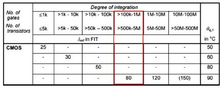
SN 29500-2:2010-09, Table 2. Failure rates for microprocessors and peripherals, microcontrollers, and signal processors7)
3) Finding the λref value
When referring to the table below for the calculation, the λref value with 986,432 (≒1M) transistors is found to be 80 Fit.
4) Finding the ΔTj value
For the calculation, refer to equations (5) and (6) of IEC TR 62380. First, substitute the ambient thermal resistance value for the PQFP 144-pin package into equation (5) for calculation. Then it is 52.54 °C/W. Where the K value is 1.4, it is the same as that of the previous example. Next, substitute equation (6) to calculate the ΔTj value. The operation conditions are the same as in the previous example, and the power consumption is 0.5 W; therefore,
ΔTj = 52.54 °C/W × 0.5 W = 26.27 °C.
5) Finding the πT value
For the calculation, refer to the vehicle mission profile in Table 1 to calculate the temperature dependence factor πT according to the operation time.
① Mathematical models for πT7):
| (17) |
| (18) |
| (19) |
where
TU,ef : θ U,ref + 273 in Kelvin
T1 : θ VJ,1 + 273 in Kelvin
T2 : θ VJ,2 + 273 in Kelvin
θ U,ref : reference ambient temperature in °C
θ VJ,1 : reference virtual(equivalent) junction temperature in °C
θ VJ,2 : θ VJ,2 = θU + Δθactual virtual(equivalent) junction temperature in °C
θU : mean ambient temperature of the component in °C
Δθ : Δθ = P × Rthincrease in temperature due to self-heating(the self-heating of CMOS circuits is also frequency-dependent)
P : power dissipation
Rth : thermal resistance(junction-environment)
A, Ea1, Ea2 : constants
② A, Ea1, Ea2, and θ U,ref values for integrated circuits: Refer to the table below.
③ Finding the Z value using equation (18)
TU,ref = θ U,ref + 273, and θ U,ref is 40 °C and TU,ref = 40 + 273 = 313 according to Table 3. Next, to find the T2 value, find the actual virtual junction temperature θ VJ,2 value. θ VJ,2, = θU +Δθ, so first, find the temperature rise Δθ due to self-heating. This value is P × Rth, so it is the same as the ΔTj value. Next, find the average ambient temperature θ U value of the microprocessor. For this, apply the three temperature values to the Table 1 motor types to come up with the values below.
SN 29500-2:2010-09, Table 9. Constants7)
θ VJ,2 (Temp.1) = 32 °C + 26.27 °C = 58.27 °C
θ VJ,2 (Temp.2) = 60 °C + 26.27 °C = 86.27 °C
θ VJ,2 (Temp.3) = 85 °C + 26.27 °C = 111.27 °C
Therefore, the T2 values are shown below, respectively.
T2 (Temp.1) = 58.27 + 273 = 331.27
T2 (Temp.2) = 86.27 + 273 = 359.27
T2 (Temp.3) = 111.27 + 273 = 384.27
When applying the θ VJ,2 and T2 values to equation (18), the values below come out.
Z(Temp.1) = 11605 × ((1/313) - (1/331.27)) = 2.0448
Z(Temp.2) = 11605 × ((1/313) - (1/359.27)) = 4.7751
Z(Temp.3) = 11605 × ((1/313) - (1/384.27)) = 6.8766
④ Finding the Zref value using equation (19)
The TU,ref value is the same as ③, so it is 313.
T1 = θ VJ, 1 + 273, and the reference virtual junction temperature θ VJ, 1 value is 90°C according to Table 2, so the calculation comes up with T1 = 90 + 273 = 363.
When applying the θ VJ,1 and T1 values to equation (19):
Zref = 11605 x ((1/313) - (1/363)) = 5.107. For reference, as Zref is the reference value, unlike with Z, the three temperature states need not be applied in the Table 1 mission profile.
⑤ Finding the πT value using equation (17)
First, the denominator is found as shown below.
0.9 × e(0.3×5.107) + (1 - 0.9) × e (0.7×5.107) = 7.7342
Second, the numerator is found as shown below.
0.9 × e(0.3×2.0448) + (1 - 0.9) × e(0.7×2.0448) = 2.0805
0.9 × e(0.3×4.7751) + (1 - 0.9) × e(0.7×4.7751) = 6.5994
0.9 × e(0.3×6.8766) + (1 - 0.9) × e(0.7×6.8766) = 19.4001
Therefore,
πT, (Temp.1) = 2.0805 / 7.7342 = 0.269
πT, (Temp.2) = 6.5994 / 7.7342 = 0.853
πT, (Temp.3) = 19.4001 / 7.7342 = 2.508
Third, to find the temperature dependence factor according to the yearly operation time of 500 h, when applying the τ1, τ2, and τ3 values in the Table 1 mission profile, it comes out as shown below.
((0.020×365×24) / 500) × 0.269) +((0.015×365×24) / 500) × 0.853) +((0.023×365×24) / 500) × 2.508) = 1.329
6) Calculating the BFR for microprocessors considering the operation phases and using equation (16):
λ = 80 Fit ×1.329 = 106.32 Fit
7) Calculate the BFR for microprocessors taking into account the non-operation phase. According to SN 29500-2:2010-09, 4.4, integrated circuits are often not subject to electrical stress during the operation time of the module or equipment. Even in this case, damage to integrated circuits may happen. To take into account the corresponding failure rate, the stress factor πW should be applied.7)
① The mathematical model for failure rates during the non-operation phase7):
| (20) |
| (21) |
| (22) |
where
W : ratio, 0≤ W≤ 1duration of component stressing to the operating time of the equipment
R : constant, R=0.08This takes into account that non-stressed components may also fail.
λ0 : failure rate at the wait-state temperature, but under electrical stress. The wait-state temperature is the component or junction temperature during the non-stress phase.
λ : failure rate under the actual operating or reference temperature, as in equation (13), (14), (15), or (16)
θ 0 : wait-state temperature in °C
② Finding the W value
The duration of the component stress due to the operating time of the equipment, the W value, is 0.058 when the τon value in the Table 1 mission profile is applied.
③ Finding the λ0 value. For this, apply equation (22).
λref is the same 80 Fit as before. In addition, to obtain the πT (θ 0) value, if the atmospheric temperature θ 0 is obtained, 10 °C, the temperature at which the vehicle does not run, can be applied in the Table 1 mission profile. Actually, the atmospheric temperature θ 0 and the junction temperature increment ΔTj are not the same. As the temperature condition in which the vehicle does not run in the mission profile is ΔT3, however, that was applied. Therefore, when πT (10) is calculated by applying it to equation (17), πT (10) = 0.0366. At this time, the non-operation time τoff is multiplied to obtain the temperature dependence factorπT according to the annual non-operation time. Then πT (θ 0) = 0.942×0.0366 = 0.0345.
Eventually, based on equation (22):
λ0 = 80×0.0345 = 2.7592 Fit
④ Finding the πW value. For this, apply equation (21).
The R value is 0.08 as a constant, and the λ value is 106.32 Fit, calculated in 6). Substituting these values into ② and ③ in equation (21), πW = 0.058 + 0.08×(2.7592 / 104.68 )×(1- 0.058) = 0.06.
⑤ Finding the λW value. For this, apply equation (20):
λW = 106.32×0.06 = 6.3792 Fit
Thus, the BFR value for the non-operational phase is 6.3792 Fit.
The following example is the failure rate for the two failures caused when 20 products were tested for 500 h in an environment with acceleration factor (AF) = 100, using the χ² (chi square) statistical function, which is mentioned in ISO26262-11:2018, 4.6.2.2.1.4) Here, the confidence level for the failure rate is 70 %.
1) Exponential model4):
| (23) |
where
n : number of failures multiplied by the correction factor
CL : confidence level value(typically 70 %)
AF : acceleration factor
2) Acceleration factor (AF):
As the acceleration factor model considering the main failure mechanism of the hardware element varies depending on the acceleration factor, such as the temperature, humidity, voltage, and vibration, it should be appropriately selected according to the acceleration test conditions. For the semiconductor life acceleration test, the Arrhenius model is mainly used. For reference, the paper titled “Evaluation Method for Functional Safety of Semiconductors for Vehicles Compliant with ISO 26262 and ISO/PAS 19451” provides an example of the use of the Arrhenius model.8)
3) Calculation of BFR
① Cumulative operating time: 20 × 500 = 10,000 hours
② Acceleration factor (AF): 100
③ χ²CL;2n+2 calculation (using Excel functions):
2n + 2 = (2 × 2) + 2 = 6, CL = 0.7
CHISQ.INV(0.7, 6) = 7.231
④ Therefore,
λ = (7.231 × 10⁹) / (2 × 10000 × 100)= 3615.5 Fit
2.5 Guide to BFR Calculation
The BFR calculation criteria for vehicle electronic components are prioritized as shown below(the number indicates the priority level).
1) Apply the BFR designated by the customer.
2) Calculate the BFR by referring to the failure rate data book designated by the customer.
3) Apply the BFR provided by the parts manufacturer. In this case, however, if the environmental parameter value (temperature/humidity, etc.) where BFR is applied differs significantly from the actual value, it should be calculated by referring to the failure rate data book specified by the customer, or to your own standard.
4) If any route is not available, it should be calculated by referring to your own standard or to the failure rate data book specified by the customer.
3. Failure Mode, Failure Mode Distribution Rate
According to ISO26262-1:2018, failure is “termination of an intended behaviour of an element or an item due to a fault manifestation,” and failure mode is “manner in which an element or an item fails to provide the intended behaviour.”3) To analyze these failures well, it is necessary to first grasp the function, which is the intended operation. This is because failures and failure modes depend on functions.
In the early stages of the analysis, the failure modes can be derived through reference documents like ISO 26262-5:2018 Annex D1), ISO 26262-11:20184), and IEC 617095). Later, however, through the judgment of experts like developers, the analysis should be complemented or newly identified and reinforced. FMEA, FTA, and DFA are very useful analysis techniques for deriving these failure modes.
The failure mode distribution rate is a ratio where only one failure mode among the total failure rates of hardware elements is involved. For example, in the case of a semiconductor die, it can be gained by dividing the area occupied by individual elements among the total areas constituting the semiconductor die, or by dividing the number of equivalent gates or transistors consumed by individual elements by the total number of equivalent gates or transistors constituting a semiconductor die.4) If the size of the transistor is not uniform, however, the number of transistors existing in the same area will be different, so it is recommended that the rate be obtained based on the number of transistors rather than on the area. As a precaution, the safety mechanism is not considered in the failure mode distribution rate at this time. This is because the safety mechanism will be considered and reflected in the implementation of FMEDA.
3.1 Guide to the Derivation of Failure Modes
The procedure for deriving the failure mode for the vehicle electronic components is set as in the following priority order(the number indicates the priority level).
1) Apply the failure mode provided by the customer.
2) Apply the failure mode described in the failure rate data book designated by the customer. This applies, however, only to devices conforming to Class I9), such as passive and discrete devices.
3) Apply the failure mode provided by the component manufacturer(the supplier).
4) If the failure mode is not available through any channel, apply your own standard or the failure mode described in the failure rate data book designated by the customer to devices conforming to Class I9). Derive the failure mode for components conforming to Class II9) or Class III9) by referring to ISO26262-5:2018 Annex-D1) and ISO26262-11:2018.4) In particular, in the case of semiconductors, the examples provided in ISO26262-11:2018, 5.1.4, 5.2.2, 5.3.2, and 5.5.24) are very useful.
5) Apply the failure modes derived from safety analyses via FMEA/FTA/DFA. In other words, apply the experts’ judgment, as shown in the examples below. Example 1): Failure mode of the CAN transceiver
a. Operation mode change is impossible(idle, sleep, or normal-mode access is impossible, and wake-up operation is not possible)
b. Diagnosis function disabled(the CAN bus status cannot be monitored, and the CAN transceiver itself cannot be diagnosed)
c. Transmission not possible(the CAN data received from the MCU cannot be transmitted to the CAN bus)
d. Cannot receive(cannot transmit the received CAN data to the MCU)
Example 2): In the case of Drift, a failure mode that exceeds the allowable error range, add Drift 0.5 and/or Drift 2 as a failure mode.
3.2 Guide for the Calculation of the Failure Mode Distribution Rate
The procedure for calculating the failure mode distribution rate for vehicle electronic components is set as in the priority order shown below(the number indicates the priority level).
1) Apply the failure mode distribution rate provided by the customer.
2) Apply the failure mode distribution rate described in the failure rate data book designated by the customer. This applies, however, only to devices conforming to Class I9), such as passive or discrete devices.
3) Apply the failure mode distribution rate provided by the component manufacturer(supplier).
4) If not available through any channel, apply the expert’s judgment or deal with it through the 1/n process(where n is the number of failure modes).
4. Conclusion
This study defined base failure rate(BFR), the main input parameter for failure mode effects and diagnostics analysis (FMEDA), to understand BFR correctly, and showed the BFR calculation methods through different examples for application in the field. In addition, it provided a guide for the methods of deriving the failure modes and calculating the failure mode distribution rates.
The findings of this study will help in deriving a more precise and accurate analysis method in performing FMEDA to evaluate the random failures of hardware.
Nomenclature
| ASIL : | automotive safety integrity level |
| BFR : | base failure rate |
| CAN : | controller area network |
| CMOS : | complementary metal oxide semiconductor |
| EEC : | evaluation of each cause of safety goal violation |
| FIT : | failure in time |
| FMEDA : | failure mode effects and diagnostics analysis |
| MCU : | micro control unit |
| PMHF : | probabilistic metric for random hardware failures |
References
- ISO 26262-5:2018, Road Vehicles Functional Safety Part 5: Product Development at the Hardware, 2nd Edn., 2018.
-
B. K. Park and S. H. Lee, “The Methods for Describe the Safety Mechanism and Estimate the Diagnostic Coverage in order to Conduct the Efficient FMEDA,” Transactions of KSAE, Vol.26, No.6, pp.791-798, 2018.
[https://doi.org/10.7467/KSAE.2018.26.6.791]

- ISO 26262-1:2018, Road Vehicles Functional Safety Part 1: Vocabulary, 2nd Edn., 2018.
- ISO 26262-11:2018, Road Vehicles Functional Safety Part 11: Guidelines on Application of ISO 26262 to Semiconductors, 2nd Edn., 2018.
- International Electrotechnical Commission, IEC 61709 Edition 3.0: Electric Components - Reliability - Reference Conditions for Failure Rates and Stress Models for Conversion, 2017.2.
- International Electrotechnical Commission, IEC TR 62380 Edition 1.0: Reliability Data Handbook - Universal Model for Reliability Prediction of Electronics Components, PCBs and Equipment, 2004.
- Siemens Norm, SN 29500, Part 2: Expected Values for Integrated Circuits, 2010.9.
- B. C. Kim and D. S. An, “Evaluation Method for Functional Safety of Semiconductors for Vehicles Compliant with ISO 26262 and ISO/PAS 19451,” The Institute of Electronics and Information Engineers, Vol.43, No.7, pp.33-43, 2016.
- ISO 26262-8:2018, Road Vehicles Functional Safety Part 8: Supporting Processes, 2nd Edn., 2018.